
This is not in the MEI style, nor is it of exam length and variety, but it was written in response to other general investigation of pollution. I have kept the material within the general syllabus constraints of Edexcel, which means it is mostly within MEI S1 and S2 too.
1 I found a graph in an academic text that compares seven megacities’ pollution index (MPI) with their capacity for generating knowledge (KIR). You can see the diagram here and read bits of the paper for yourself here. [Link easily lost, sorry]
The data pairs are given as City (KIR, MI): Tokyo (0.9, -0.3), New York (1.15, -0.2), Mumbai (0.6, 0.4), Shanghai (0.25, 0.9), Los Angeles (1.5, -0.25), Osaka (0.85, -0.4), Beijing (0.6, 2.05).
i Plot a graph of these points. [2]
ii Calculate a product moment correlation coefficient and comment on the level of correlation. [5,2]
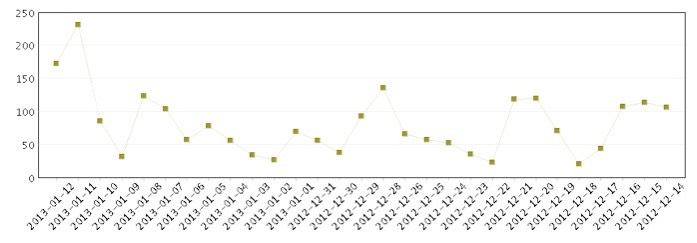
2 The graphic above, from http://datacenter.mep.gov.cn, shows PM10 coarse particle pollutant levels as measured in Beijing for a period of 29 days. Abstract the data; produce a two-sided (unordered and ordered) stem and leaf diagram; draw a boxplot; find the mean and standard deviation. [3, 3, 5, 4]
Comment and identify any outliers. Lastly, criticise the graph given. [1, 1]
3 The same source gives historic data. For the 88 days from 14/10/2012 to 12/1/13, I give you these partial results: Σx = 6634, Σx2= 652806. Show that the mean and standard deviation add to 117. [5]
Assume the distribution is roughly normal [it is] and hence declare outliers to be more than two standard deviations from the mean. Explain why there can be no low outliers. Comment on there being 6 values over 150, the la(rge)st three of which are 163,174, 232. [1,2]
Given that 67 and 71 are the 44th and 45th data points, attempt to comment on skewness of the distribution. Excel says the skewness is close to one, where a Normal distribution has skewness of zero. [2]
4 Assume that a similar period to that of Q3 is normally distributed as X~N(75, 402). Find
the probability that X is between 100 and 150, P(100<X<150) and use this result and others to band the whole distribution in sets of fifty from 0 to 250, showing the percentage in each category. [2,6]
5 The value used at BSB to curtail outdoor activity is an AQI of 250. A researcher says that the mean AQI for January 2013 was 199. If we lost 20% of days to high pollution, show that this places the Std Dev at about 61. If the Std dev was 50, what % of days would you expect to lose? What about an s.d. of 70? [2,2,1]
We’re assuming that weekends are no different from weekdays.
The annual mean for AQI is steadily improving: the last three year’s means are 160, 151, 145. What do predict 2013’s to be? [work for the second mark, please] [2]
6 The data used in Q2 gives figures for weekends only as n= 24, Σx = 1756, Σx2= 171260. Find the mean and std.dev. for weekends and show that the difference between these values is 31. By subtraction, find the values for weekdays. Do these results support any suggestion that day is correlated with pollution level? What would you want to do to test that? [2,4,1,1]
Here are mean and std dev for the seven days:
day Mon Tue Wed Thu Fri Sat Sun
mean 54.4 87.6 89.7 72.7 80.1 88.7 55.7
Std Dev 23.0 52.2 43.9 33.3 37.2 38.9 38.7
count 13 13 13 12 12 12 13
Do regression analysis on the displayed data and make comment on the correlation figures you produce. [6,2]
Make some other comments directing more research. You can investigate more of this data for yourself here . (There’s a start date near the top where you can choose a month, click Update and then the magnifying glass image; no doubt it is easier to follow if your Chinese is good enough. It will copy to Excel.)
y=1.4-1.4x within the ability to estimate values from the graph. r= -0.618, n=7 on my calculation. So weakly negatively correlated and not quite significant., as if connected to other factors - a likely condition. Valid to say that pollution lowers the ability of a city to generate knowledge, since there is no counter-example. You might argue that Beijing is exceptional; that would be because the push to work in the capital exceeds the push to work in a ‘better’ environment, as happens in, say, the USA. Why work in NewYork if you could would in Massachusetts? Why work in LA if you could work elsewhere in California?
An AQI of 250 equates to 385 µg/m3. It is an awkward conversion process between scales.
[Note that std dev is the second moment, skew (as defined in modern texts) is the third moment, and kurtosis is the fourth. Moment is distance from the mean; second moment is the geometric mean of the squares of the distance from the mean. In Mechanics there are equivalents, inertia is the second moment (M3 in Edexcel, ordinary FM at CIE, M5 at MEI). Karl Pearson’s first skewness coefficient is (mean-mode)/(std dev) and his second is 3*(mean-mode)/(std dev). These are found in A-level Stats, sometimes. It occurs to me that some simple transformations should be available to skew the normal on demand and hence to match a distribution to all the convenient theory; the theory I found says these exist, but they are not as simple as I had expected].
academic paper on pollution and knowledge found at https://davies60mathematics.wikispaces.com/file/view/Pollution+and+Megacities+(Correlation).pdf or google ‘megacity pollution KIR’
