
Following on from Coronavirus, which is a matter of immediacy today, I'm going to try to provide a more basic approach to the study of this sort of modelling.
Daniel Bernoulli, way back in 1760, did some thinking on this, based on data collected most of a century earlier by John Graunt [1]. A suitably simple model for school-level study supposes that a cohort of individuals born in a partiucular year has an age-specific death rate µ(t) at age t. Then, given an initial population X₀, whose size, X, s expressed by the function x(t) then
dx/dt = - µx which is a product of functions in t. By separation of variables we get something very like the expression for integrating factors in the pages on differential equations, that x = X₀ exp( - integral µ(t) dt = X₀ exp(H(t)) where we could call H(t) some sort of accumulated hazard. [1, P3]. This gives an idea of a general form of the expected modelling equation.
In general ther is a birth rate and a death rate, whose difference is expressed by function µ. What happens in populations is that different factors affect the two parts, so they are often indicated separately. I have written sevaral pages on related topics; essay 208 and 240, but also essays 173-5.
Looking at very simple models we might postulate a fixed population, so that we declare the birth and death rates to be equal or zero. Then a disease causes a loss, and we have a model very similar to dx/dt = - kx where k is the infection rate.
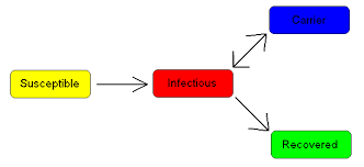
Quite clearly during the progress of a disease the total population is made up of three groups, where I have given the usual labels—taht is, I called them something different at first but then found a text that agreed with what I'd scribbled.
S, those at risk of catching the disease, to be thought of as Susceptible
I, those currently infected, who are able to pass the disease to the susceptible group. I have used the character 𝙸 below to help it be distinguishable.
R, those who are removed from the infection, either by recovering or by immunisation or by dying. These are the people who cannot pass the disease on.
Obviously the total populationN, is N= S+I+R where each of S,I & R are functions in time.
This idea leads us to the idea of the reproduction number, usually denoted R₀ which represents the number of people each infectious person will infect. R₀>1 causes the disease to spread; R₀=1 represents an endemic disease, since each infected person infects one other, so the population infected stays constant; R₀<1 means the diease dies out.
The commonly chosen variables are:
(i) something to represent how fast people become infected. We use 𝞫 to represent the number of people each infected person infects per time period. While it is not true, we assume that all people are equally likely to contract the disease. So in any time unit each infected person is able to transmit the disease to 𝞫N others. The only others who may contact the disease is the fraction S/N. The fraction of the population removed from reg susceptible group are those infected, so I think dS/dt is the product of 𝞫N, S/N and 𝙸/N, and that therefore dS/dt = - 𝞫 S 𝙸 / N which seems dimensionally consistent with a rate of people per time unit.
(ii) something representing the death or recovery rate, which we could perhaps also view as the time to a result. T o be consistent with 𝞫 we want a rate, so the convention is to use 𝞬 to indicate the rate at which we gain a result (either death or recovery). Since trhat will be in people per time unit, the reciprocal, 1/𝞬, is useful in time units per person and represents the mean infectious period. This suggest sa fairly simple model where R₀ is simply 𝞫 /𝞬. The infectious period can create difficulties. Within the SIR model for the time being, we can see that dR/dt = 𝞬 𝙸
Since N=S+I+R was a fixed population, dN/dt=0 = dS'dt + d𝙸/dt + dR/dt and in the absence of an alternative, d𝙸 /dt = 𝞫S𝙸/N - 𝞬𝙸
As {2] points out the notion of a fixed population succeeds here if infection is very much quicker than the rates of birth and death (which you might construe mathematically as competing infections). So other versions of the SIR model treat the cases where births and deaths are considered, those where there is no immunity, or where immunity can occur in births or where immunity is not permanent or, perhaps the most worrisome, where there is a period in which the infected person is not yet infectious.
Another, simpler model simply says that the susceptible is everyone that is not currently infected. that gives d𝙸/dt = 𝞫 𝙸 (1- 𝙸) which is a standard A-level problem where ln ( 𝙸 / (1- 𝙸) = c + 𝞫 t. You supply initial conditiona and express 𝙸(t).
A slight imporovement gives d𝙸/dt = 𝞫 𝙸 (1- 𝙸) - µ 𝙸 where the µ 𝙸 term represents some people being or becoming immune. This leads to the population being as infected as it can be without reaching unity, that is, the first differential has a later zero value. In this model R₀ is, I think, 𝞫/µ.
I hope to return to this topic armed with better tools.
DJS2020127
top pic found hurriedly via Google, but I'd prefer the red box to be labelled Result, Resolved or Removed.
2 https://en.wikipedia.org/wiki/Mathematical_modelling_of_infectious_disease
3 https://www.slideshare.net/IgnasiGros/delaydifferential-equations-tools-for-epidemics-modelling
I was hugely frustrated that much of what I wanted to read was hidden behind pricing barriers which do not exist for those employed in academia. So much for 'information wants to be free'. I would see this as an exciting module within a university course, lending itself to extensive modelling, not least those extensively using computing power. DJS 20200127
I found [3]. with which I disagreed with quite a lot of the maths as shown, especially slide 21. Slide 37 is dimensionally rubbish unless the declared 𝞪 andf 𝞫 have different units. However, slides 40-45 and 46-55 do show how to model incubation periods, delayed infectiousness and the asymptomatics (possible carriers).
Q1 𝞪 = 𝞫 suggests to me that both are zero. This is inconsistent with Bernoulli saying a = b = ⅛.
Q2 𝙸(t) = ( 𝙸₀ exp( 𝞫 t) ) / ( 1 - 𝙸₀ + 𝙸₀ exp(𝞫 t) ) very clumsy to type without use of script editors.