
Start from the modelling in Growing Up, dy/dt = y(1-y), the standard growth curve. Gowth depends on what there is and what is left, with target growth to be unity. That gives y = ( 1+e-t ) -1.
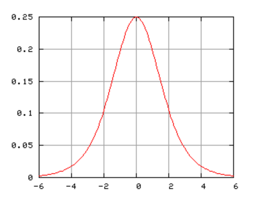
This is the distribution function for the Hubbert curve, so differentiate and you have what I show next.
The Hubbert Curve is a ‘symmetric logistic distribution curve’, which is distinct from a gaussian function.
![]()
As I wrote at the foot of Peak Oil [essay 100, late 2012], I agree that we would expect a bell-shaped curve, but I’m surprised we’re not assuming Normality. I’m satisfied that the peak be symmetrical but question the assumptions behind that choice. The curve is produced in a sort of self-predicting way by requiring that the curve be bell-shaped (hence the divisor term, (1+ae-bt)² with the maximum (a single maximum is required) as the numerator, let’s say Ke-t. You don’t have to play with this much (or² maybe you do; try it) to see that the year of maximum production is b-1 ln(a), that you can force K to be unity, but K is the total recovered (resource, oil in this case).
I think this may belong in my economic modelling section. I am surprised not to find lots of argument over the requirement for symmetry of the model; I am surprised to see a meek acceptance of the modelling thinking. Why is the curve not skewed negatively to reflect demand outstripping supply? The symmetry presupposes a replacement energy source always being available. Yet if we looked at total energy demand, surely a skew is required (until we reduce demand, or population, or both)? Obviously (well I think it is obvious), we would need to sum a series of curves to model multiple events — but the underlying assumptions are not being questioned. There are parallels with cash-flow modelling; summing curves is ‘easy’ in computing. A partial answer to my issue here is that, as wikipedia puts it: A post-hoc analysis of peaked oil wells, fields, regions and nations found that Hubbert's model was the "most widely useful" (providing the best fit to the data), though many areas studied had a sharper "peak" than predicted.
Start from dy/dt = y(1-y), the standard growth curve (growth depends on what there is and what is left, target growth unity). That gives y = (1+e⁻ᵗ)⁻¹. If your target is h then rewrite this using proportions; let y=x/h and dx/dt = x(h-x), or perhaps (h-x)x/h (check that!). This is the distribution function for the Hubbert curve, so differentiate and you have what I show next. CIE FM Stats has a use!!
You might read https://klemow.wilkes.edu/Hubbert.Curve.html on Hubbert Curve and Peak Oil.
Another answer, arising from the writing I did for Growing Up, says that the reason is one of analysis – given some data, we can successfully fit a growth curve or Hubbert curve (we can fit it exactly; we can do some maths and find the constants required). Doing this with the Normal distribution is necessarily an approximation to something (discuss? please?). Since the integration that gives us the Normal is one we cannot do (Liebnitz proved that, I think), we would end up ascribing meaning to the standardised variable and hence to mean and variance of the apparent distribution. It seems to me worth doing, but if the two curves are sufficiently similar (meaning that the difference is smaller than the error in the model, I reckon) maybe nobody cares enough to do it. Project, anyone?
² not squared, footnote. I did the differentiation and had an extra ln(b-1) I couldn’t get rid of. So, feeling stupid, I tried different thinking: The assumption that the curve is symmetrical requires the peak to be when t= b-1 ln(a), hence xmax = K/4 e-1/b . Please check that and tell me you do or do not agree. A ‘plot’ of the Hubbert curve puts 0.25 as the peak, assuming all constants to be unity. We can choose t=0 as the peak to confirm that the peak is at xmax =K/(1+a)², so if a=1 this is K/4. You might (please) make comment before I try to turn this into a Maths page. (Oh, you didn’t; what a pity).
I think there ought to be separate page on epidemics, which I eventually began in early 2020.
Q1. Starting from the dy/dt = y(1-y), show this gives y = ( 1+e⁻ᵗ ) ¹ and state the intial conditions. Differentiate y = ( 1+e⁻ᵗ )⁻¹ , produce dy/dt as a function in t and express this in terms of e⁻ᵗ.
Q2. Use cosh t = (eᵗ + e⁻ᵗ)/2 to express the Hubbert curve in terms of cosh t.
Q3. Show that 1+ cosht = 2 + 2cosh² t/2, and hence that the Hibbert curve has a third form, ¼ sech² t/2.
Q4. In the original of this page I wrote If your target is h then rewrite this using proportions; let y=x/h and dx/dt = x(h-x), (check that!). This is the distribution function for the Hubbert curve, so differentiate and you have what I show next. CIE FM Stats has a use!! But when I tried this at home (famously dangerous) I had an extra factor of 1/h, that is, dx/dt = (h-x)x/h. Then I wondered what I had meant by your target is h, where I'd been assuming that h was the target height, but height of what, the peak of the Hubbert curve or the distribution function? Perhaps someone will elucidate.
A1 at t=0, dy/dt=0 Your result is symmetrical about t=0 and the curve's maximum is at t=0, y=¼.
2 not squared, foot note. I did the differentiation and had an extra ln(b-1) I couldn’t get rid of. So I tried different thinking: The assumption that the curve is symmetrical requires the peak to be when t= b-1 ln(a), hence xmax = K/4 e-1/b . Please check that and tell me you do or do not agree. A ‘plot’ of the Hubbert curve puts 0.25 as the peak, assuming all constants to be unity. We can choose t=0 as the peak to confirm that the peak is at xmax =K/(1+a)², so if a=1 this is K/4. You might (please) make comment before I try to turn this into a Maths page.
This page revisited and quite a bit rewritten on 20211119. Long retired, so not so quick on the actual maths!!