
Suppose we have a disease like ordinary influenza, where each person who gets sick infects 2 other people. Suppose the period of infectiousness is five days, then after thirty days we've had five cycles and potentially that one infected person has infected {2,4,8,16,} 32 others; After sixty days, ten cycles, this is 1024 infected people.
1. Looking at ten cycles then, find how many infected people there might be if the infection index (the two above) is instead:
1. a) 1.4 b) 1.5 c) 1.9 d) 2.5 e) 3 f) 4
The page on epidemics explains that the index figure is usually referred to as R₀, which is the mean number of people that one infectious individual goes on to infect. This is also called the reproduction number. After a while, not only does the disease generally fade, but the population able to catch the disease rises. Once R₀ falls below unity, the disease will die out. However, if the population is highly mobile, then the local effect may die out, but new infections occur.
Imagine we have a population of 100 and a reproduction number of 4; after 4 cycles we have 32 new infections but these add to a total of 61 people who have been infected. So in the next cycle the expected number of infections exhausts the population; everyone has it (or has had it) and no more people can be infected.
2. Consider a population of 1000 and the range of R₀ values given in Q1. Find the number of cycles to exhaustion.
There's a subsidiary problem here: using r for R₀, we want to add 1+r+r²+r³+r⁴+... where 1 occurs a time 0. This sums to S= (rⁿ-1) / (r-1) and we want to find the first value of n that makes S>1000. Manipulating this to calculate n (and then round up to the next integer), requires logs. Show that rⁿ > 1000(r-1)+1 (=T, say) and calculate n by doing log T / log r.
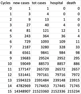
Now suppose that everyone who gets the disease is infectious but unaware of this; they are asymptomatic for much of the infectious period. Of those who catch the disease, let's say x = 10% need to be in hospital and of these, as much as d = 10% die. So that is dx= 1% mortality, those that catch the disease and die from it. Now let's assume we have a disease of reproduction number 3 and look at what happens, shown to the right. At cycle 10 we have a national problem and at cycle 13 we are going to have many more needing to be in hospital than we can put there. That column is not 'in hospital' but 'has been in hospital'.
Suppose that we are able to reduce the infection rate from 3 to 1.5, but that we don't change the situation until we have 6000 new cases (cycle 8). Then this is what subsequently happens, on the left.
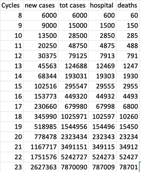
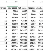
Look what reducing the reproduction number to 1.5 from 3 does to cycle 13; 1.6 million cases becomes 45 thousand; the deaths go from 24 thousand to 12 hundred, twenty times less. By cycle 23, 26 million cases, even a country the size of the UK is going to have difficulty spreading the disease among the population, as the number recovered (and temporarily immune) has become such a large proportion of the population that the reproduction figure is going to drop, simply becasue the people available to be infected is not available. Because the effect of this sort of growth is so explosive, a small effect on the reproduction number has a huge effect on the figures. On the right I show the figures on reducing only to 1.4. Look at line 20, where the number of new cases is already less than half those that would occur if R₀
3. Create a similar spreadsheet to mine and look at values of R₀ from 1.7 to 1.1 by changing the figure in the top row. Assume a change of R₀ from 3 to your value occurs at cycle , at 3000 known cases, not as above, and declare the cycle in which deaths pass 10,000. While R₀ was 3 this occurred during cycle 13.
Now view these numbers as demonstrating when capacity to cope with hospital cases is exceeded. At this point, suddenly the death rate rises dramatically. At cycle 8 we had, in theory a hundred deaths and a thousand in hospital; it probably takes some time to cause a change in the reproduction number, but hopefully that is less than a whole cycle. If a cycle is the same as a week, you have a strong idea how fast the situation changes. Once the case load passes 50% of the total population, matters change (but this is complicated to do and I offer it as a challenge to share)—in effect the reproduction number is changed as described above. Note below on this.
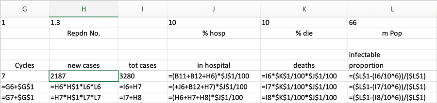
If you view the reproduction of disease as being a probability and the mixing of the population making the probability of passing the infection equally likely (not true but we need assumptions to have structures we can model) then the number of people infected by anyone else depends on the number of infectable people that are met, so that the reproduction number needs to be multiplied by the probability that the infection can be passed. Multiply R₀ by uninfected/population. I found that this factor was not large enough to produce the effect I expected.
I can insert this into the spreadsheet. I've set the population at 66 million. The spreadsheet model needs improving; lets us assume that the hospitalised are there for three cycles. At the moment, this model predicts that 1% of the population will die whatever we do, because we have no cure available. We need the reproduction number to fall so that not everyone gets the disease.
• Leaving R₀ at three during cycle 16 the total cases passes the population total and we peak at 6.3 million somehow 'in hospital', which means hugely more deaths. If we decide that hospital saturation is 100,000 beds, saturation occurred in cycle 11.
• Failing to reduce R₀ by much, say to two, we peak at cycle 21 and hospitals saturate early in cycle 16, wishing we'd changed behaviour much sooner. Total cases about 57 million.
• Reducing R₀ to 1.5, we peak at cycle 33 (17 cycles later than R₀=3) and the hospital system copes somehow up to cycle 21. Total cases about 41 million, 62% of the population; so total deaths about 400 thousand.
• Reducing R₀ to 1.4, we peak at cycle 32 (yes, earlier, just) and the hospital system copes until late in cycle 23, 54% of the population having had the disease and about 50 thousand fewer deaths. If the cycle is 5 days, that puts the peak at six months from start.
• Reducing R₀ to 1.3, we peak at cycle 38 and the hospital system copes into cycle 35; we're down to 44% having had the disease and deaths are under 300 thousand. At cycle 65 we will have probably relaxed the restriction and thoroughly changed our ways. But at a 5 day cycle that is a whole year in the future.
• Reducing R₀ to 1.2, we peak at cycle 48 and the hospital system copes to cycle 37, peaking at 310 thousand cases. Total cases would be 21 million 32% of the population with a death toll of 213 thousand. We are not yet aware what we need to do to reduce R₀ to this low level.
So you see that the reduction of R₀ is critical. When the change in R₀ value occurs makes all the difference. To make the model reflect what should occur, a steadying of the load at hospital, several things could occur:
(i) cases remain in the community,
(ii) behaviour changes so that the infection rate reduces still further
(iii) the model is improved to reflect that infection reduction. I tried squaring the effect of the infectable population: this produced the strength of effect I was expecting to see, reducing deaths at R₀ =1.5 to 234 thousand, peaking in cycle 28, but still far far too many hospitalised cases, over 700 thousand. This suggests that we need to be able to change R₀ as needed towards values around 1.3.
DJS 20200324
1. This is n¹⁰, where n is the index, so, to the nearest integer a) 29 b) 57 c) 613 d) 9,536 e) 59,049 f) 1,048,576
2. There's a subsidiary problem here: using r for R₀, we want to add 1+r+r²+r³+r⁴+... where 1 occurs a time 0. This sums to S= (rⁿ-1) / (r-1) and we want to find the first value of n that makes S>1000
a) 18 b) 16 c) 11 d) 8 e) 7 f) 6
3. Pairing (R₀, n): (1.9,15); (1.8, 16); (1.7, 16); (1.6, 17); (1.5, 18); (1.4, 20); (1.3, 22); (1.2, 27)
Here's how I made the spreadsheet work. Yes, I should have used Names, but I didn't; small apologies.
Essay 293 - Covid-19 charts charts published daily reflecting concerns and issues.
Essay 291 - Effects of an outbreak what it says, effects, but some description of what we have (and not)
Coronavirus (Y10+) modelling problems
Epidemics more general theory
Infectious disease looking at the 2020 problem, particularly effects of the reproduction number changing.
Viruses are very small
Incidentally, I found some comparison data here, at the foot of that page:
- Every year an estimated 290,000 to 650,000 people die in the world due to complications from seasonal influenza (flu) viruses. This figure corresponds to 795 to 1,781 deaths per day due to the seasonal flu.
- SARS (November 2002 to July 2003): was a coronavirus that originated from Beijing, China, spread to 29 countries, and resulted in 8,096 people infected with 774 deaths (fatality rate of 9.6%). Considering that SARS ended up infecting 5,237 people in mainland China, Wuhan Coronavirus surpassed SARS on January 29, 2020, when Chinese officials confirmed 5,974 cases of the novel coronavirus (2019-nCoV). One day later, on January 30, 2020 the novel coronavirus cases surpassed even the 8,096 cases worldwide which were the final SARS count in 2003.
- MERS (in 2012) killed 858 people out of the 2,494 infected (fatality rate of 34.4%).
- The case fatality rate for SARS was 10%, and for MERS 34%.
- The novel coronavirus' case fatality rate [CFR] has been estimated at around 2%, in the WHO press conference held on January 29, 2020 [16] .
- [their figures, my words] Figures for R₀ for Covid-19 vary: on Jan23 the WHO says between 1.4 and 2.5; other studies say 3.6-4.0 and 2.24-3.58. For comparison, the Ro for the common flu is 1.3 and for SARS it was 2.0.