
For many things that grow, the rate of growth depends upon the amount of growth made and the remainder left to be grown. That is sufficient description for you to write a differential equation as a model. If the total (call it adult) growth is one (unity) and the amount grown at the moment (now) is x, then the amount left to grow is 1-x and so
dx/dt = kx(1-x).
Looks easy, doesn’t it? Did you do that yourself, or just read on and say “Yeah”? That is so easy to do – and it is surprising how hard people find it is to turn words into equations. I suspect I will write more of just that.
Separation of variables lies within the ordinary A-level syllabus, (possibly all of them) so, starting from the position described above:
1. Separate the variables (put all the terms including x on the same side of the equation), find some partial fractions and do the integration.
Show your answer can be written f(x) = Ae-kt and thence (from there) x = (1+Be-kt)-1
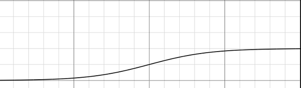
You ought to sketch the solution, but that is included in the next question. I offer here x=(1+e⁵⁻ˣ)¹ for 0≤t≤10, so you can see it is roughly the right shape.
2. A baby is 65cm at birth (t=0.75 years) and grows to full height of 180 cm at say t=20. Sketch the curve (possibly using a gadget of choice) and make comment based on what you have observed for yourself – is this a reasonable model?
3. For the case in Q1, assume x=0.5 at t=0. Decide whether this function is odd or even.
4. Assume that at t=18 you are close to your full height, say 98% of it (172cm of 175.5, for example). Assume that you were 60cm at birth and this time let us call that t=0. Show that B = 1.925 and find k. Be clear that x is not height, since the model requires it to be in the range 0≤x≤1.
5. Suppose instead that you define the differential equation as dx/dt = kt(1-t) so that the gradient of the curve depends on how much time has passed and how time time there is left. Assume that the result starts at the origin and show that y is of the form Kt² (3-2t), 0≤x≤1. This is another S-shaped curve.
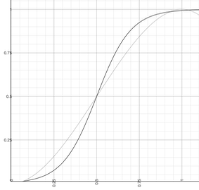
I show here 1/y = 1+e⁵⁻¹⁰ˣ = 1+ e^(5-10x) and on the same graph y = x²(3-2x). They almost meet at (0,0) and (1,1)
6. By looking at the difference between these two functions, find where they truly meet, to 3sf.
I spent some time wondering how to find the maximum gap between these two curves. I leave it as a challenge, perhaps for the better double A-level student. I think that one might write an expression for the normal to the simpler curve and then an expression for the length of the connecting line in that direction. I am not sure that the normal to the exponential to the quadratic would be the same line but, they were the same, then the gradients would be equal and the lines parallel. I find that an attractive argument, but that is not the same as solving for (x,y) where the gradients are equal. The mixture of functions drags me back to a numerical solution not an absolute one. I'd like to hear of better methods. It strikes me that perhaps some graphing packages will simply measure this.
Consider a population of size N in an environment suitable for population K. The rate of growth depends upon (is proportional to) the proportion of population we have and the proportion we have remaining to capacity. Let x=N/K and see that this is the same equation as before. No, you have to write something at this point.
The value K is called the carrying capacity. Historically in this model we use r (which I think a poor choice of symbol, but there we are) as the constant, so
dx/dt = rx(1-x) = r N/K (1-N/K).
The argument says that as N/K approaches the limit, so resources such as food or living space become critical. At stability the population is called mature (it has finished growing) and other factors—hence other models—apply. Species are described as using strategies for r or for K (r-strategist, K-strategist). To a mathematician, it is obvious that lim(N) = K as t heads to infinity. If N₀is the initial population (meaning when you start the model, then N = K N0ert / (K + N0(ert - 1)) follows in a straightforward way you can do for yourself (not hard at all after the other work, you might even say “Obvious”).
There’s an extension of this model that says the carrying capacity, K, varies with time; an obvious example is the cycle of the seasons, making K periodic. If the period is T, then K(T+t) = K(t) describes the situation.
There may also (or separately) be a delay (d) reflecting how population reacts to environment, so that K(t) = f(N(t-d)). This rapidly gets complicated, what one source I was reading calls a ‘rich’ behaviour – by which is meant that there are many possibilities reflected in the solutions. This would be a good topic for university-level research, such as in ecology. It specifically lends itself to computer-based modelling.
The collection of curves called logistic functions are found (well, almost found) in the FM Stats course; even ordinary students of Stats recognise z= (x - mean) / std dev as the standardised mean (yes you do, this is how you handle the Normal Distribution). If I use s for std dev then the probability density function f(z) = e-z / s(1+e-z)². Yes, I know s is a dependent variable too, but I’m trying to make it readable and not use mu, x and s.
7. FM students should prove that f(z) above = 1/4s sech² (z/2). Oh, yes you should, since it is a common exam-type question, likely also found on STEP papers.
8. FM students can explain (and A-level students can simply integrate, for practice) the exponential f(z) to see the Cumulative function F(z)=(1+e-z)-1. Or is that F(z)=(1+e⁻z) ⁻¹ ?We have seen this already on this page.
9. FM students should integrate the sech form to 1/2 (1+tanh(z/2)). Exam Q hint, again.
10. Students of other disciplines and those who see Maths as a tool for actually doing things should write themselves a list of things which might be productively modelled by logistic distributions. Think of the S-shaped curve of the cumulative function.
I’ll offer some less likely ones, leaving you a wealth of opportunity to write to me about;
(i) the money sent on a project, especially in construction; subsidiary parts of the same project follow the same curve;
(ii) as a substitute for the Normal distribution, since this curve can be solved analytically and is very similar (define similar?);
(iii) the Hubbert curve (see next page, and Dying Away).
(iv) Lots of thingks biologic —thingks is a cross between things and thinks—, such as sorts of epidemic.
A3: B=1. The exponential term cannot be negative, even if t could be. When t <0 the resulting exponent is the same as the equal value of opposite sign, so f(t) = f(-t), which is even.
A4 If the model x = (1+Be-kt)-1 is suitable, then at t=0, x=1/(1+B), so if x(0)= 60/175.5 =>B=1.925 => k=0.253, I think. Please confirm that you agree. (0.25256 to 5sf).
A5: This is direct integration y = k ∫ x(1-x) dx = k(x²/2 - x³/3) + c and passing through the origin makes c=0. Let K=k/6 and I think you're done.
A6: I did this by decimal search, starting from x=±0.1 and using the symmetry around (0.5,0.5). I found that the two points near the origin are (0.0675, 0.01305) and (-0.0385, 0.00456), so therefore the other two points are (1.0385 0.99544) and (0.9325, 0.98695). These both checked out as close to the implied precision. Your answers will be more rounded than these.