
Statistics is the skill (art, science, etc) of reduces a pile of data to a memorable few items — statistics are those memorable bits. Think of this as sound-byte maths.
There are two classes of measure, location and spread. In a sense, location is primary; spread is secondary information.
Location:
You know the word average; well, there are at least three of these,
mean — add them up and divide by how many, the arithmetic mean. Actually there are other means, such as the geometric (multiply all and take the nth root of n numbers) and the harmonic mean (works for speed; divide the number of values by the sum of their reciprocals). Only the arithmetic mean is in GCSE.
median — put them in order and find the middle one. Take care here, as position counts from one, so the position of the median is (n+1)/2 once they're in order. Convention is to interpolate between two middle values.
mode — look for the most common example. The example below has a mode of two, illustrating that mode is useful with large populations. ¹
Example: {1,2,2,3,5,6,7,10} has a mean of 36/8 = 4.5, a median of 4, half-way between the 3 and 5, and a mode of 2. ³
There are other measures of location included at GCSE level. You use cumulative frequency graphs to find the positions of the quartiles, positions (n+1)/4 from each end [or 1/4 and 3/4 of the way through the data]; these are also location measures. They're called the lower quartile and the upper quartile, obviously, the gap between these is in spread, below. Example {1,2,2,3,5,6,7,10} has LQ at position 9/4, value 2 and UQ at position 3x9/4=27/4=63/4, value also 6.75.
Add some value (c, say) to all data, and the location moves by the size of the translation,
x➞x+c. Multiply by a factor (m, say) and the location measures expand directly. Location measure x is turned to y by the transformation y=mx+c. You have seen this in exploring straight line graphs, which is why it is called a linear function and such a conversion is a linear manipulation.
Example: {1,2,2,3,5,6,7,10} convert by tripling it and adding 100, becomes {103,106,106,109,115,118,121,130} has a mean of 100+3*4.5= 113.5 [I didn’t work it out as 908/8] a median of 112, half-way between the 109 and 115, and a mode of 106, 100+2*3. The quartiles would be at 106 and 100+3*6.75=120.25.
Spread:
Like middle-aged spread and peanut butter, not location (butter side down), but how the data is arranged around the location measures. So when you’re worried about choosing one of the averages because they differ, you know that spread has become a consideration.
Range - simple, the gap between lowest and highest value. Don’t quote both numbers, just the gap.
Interquartile range, IQR = the upper - lower quartile values. Do not quote both numbers, just the interval. Half this is also used, the semi-IQR. See also footnote ². The IQR is the range of the middle half of the data. IDR, or inter-decile range, counts from 1/10th to 9/10th of the data, the middle four-fifths. This is pretty useless unless there is a lot of data, more than 100 items.
Example: {1,2,2,3,5,6,7,10} has a range of 9 (=10-1), an IQR of 4.75, 6.75 - 4. The IDR is a pretty silly thing to do but makes a point about interpolation: it would be the difference between positions (8+1)/10 and its corresponding point at the other end, 7.3-1.9 = 5.4
At the far end of the GCSE is the use of standard deviation. This looks at deviations, the difference of each item of data from the mean. Obviously they add up to zero, so to measure spread we find the geometric mean (square all the deviations, add them up and square root the total). This will have the same units as we started with, conveniently. It is a good challenge in calculator precision.
Example: {1,2,2,3,5,6,7,10} has a mean of 4.5 above, so deviations are {-3.5,-2.5,-2.5,-1.5,0.5,1.5,2.5,5.5} whose sum = -10 +10 = 0. The squares all end in 0.25 and the integer parts are {12,6,6,2,0,2,6,30] so the sum of squares is 64+8/4=60 and the standard deviation, the std. dev., written as a little sigma, unicode 03C3, σ, and equal to √(66/8), √8.25 = 2.872.
Using my calculator set on SD mode, STAT not REG, Σx² = 228, Σx=36, std dev σn= √8.25 = 2.872. There’s a nice short cut from the next page that says I can use 228/8 - 4.52 to get σ², (sigma squared) called the variance, the 8.25 figure in my example here.
Add some value (say c) to all data, and the spread does not change. Multiply all data by a factor and the spread measures expand. Spread measure x is only affected by enlargement, using the language of transformations appropriately. How it is affected depends on the measure, but generally the change is in direct proportion; multiply by the same factor m in y=mx+c above.
Example: {1,2,2,3,5,6,7,10} convert by tripling it and adding 100, becomes {103,106, 106,109,115,118,121,130} has an IQR of 3*4.75 = 14.25, [check: 120.25-106=14.25] and a standard deviation of 3*√8.25 = √74.25 = 8.617, checking gives Σx2 = 103652, Σx=908, µ=113.5, σn= √74.25 = 8.617 as expected. Doing this calculation the other way, starting from the bigger numbers {103,…} and changing to the simpler numbers{1,2,2…} is called coding. It is a skill that is disappearing because we all have calculators to hand. Exam boards disagree, hint.
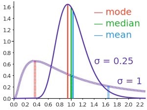
You ought to have already spent some time thinking about how it is that averages can be different. This diagram shows two distributions—the lack of symmetry is called skew and the more skew, the further apart the averages will be—you may even more than one mode. Generally, the more skew, the more you want the mode as your preferred average (though some will still prefer the median). For symmetric distributions the mean is usually preferred, but I wonder whether that is because people who can’t remember what a mean is (and who never appreciated the differences) default to the arithmetic mean. Diagram link.
DJS 20130211
small edits 20141023 and 20220523
1 Population here means the all the data; all possible data of this type is the parent population. E.g. you’re looking at IQ in school, your sample is the people you find numbers for, the population is the data you used, the parent population is the whole school, or all school age people in Britain or wider, as appropriate to your conclusions.
2 There is some more advanced work that connects IQR to standard deviation. The assumption is that the spread is roughly symmetrical, then roughly ‘normal’; if so, the IQR will be close to 1.35 σ.
3 For fun, and to encourage play with your calculator, the geometric mean is 3.55 and the harmonic mean is 2.72.
